Valuation Methodologies

Once you understand how a waterfall distributes proceeds, the next question is how to value each class of equity today before any sale has happened. The AICPA outlines several equity allocation methods for this purpose. This page walks through each one and explains where the Discounted Future Proceeds Method fits.
The Foundation: Business Value Methods vs. Equity Allocation Methods
Valuing multi-class equity is a two-step process. First, a business value method establishes the total value of the enterprise using the Cost Approach, the Income Approach, or the Market Approach. Then an equity allocation method distributes that total value across each class of equity. The methods below are allocation methods; they take the total enterprise value and determine what each tranche is worth.
What the AICPA Guidance Requires
The AICPA’s Valuation of Portfolio Company Investments of Venture Capital and Private Equity Funds guide, known as the PE/VC Guide, sets the standards for this work. Three principles stand out. First, value should be viewed from the perspective of market participants’ required rate of return. Second, valuation is fundamentally forward-looking and must consider future conditions, including access to future capital and expected dilution. Third, value should be allocated between equity and debt positions consistent with the overall valuation premise and time horizon.
Method 1 of 3: Current Value Method
The Current Value Method allocates value based on what each class would receive if the company were liquidated today. It is straightforward to apply.
Its limitation is significant. The Current Value Method is typically ignored in valuations of multi-class equity or convertible debt for companies that are not selling immediately. It does not account for the time to sell or the required returns for each class, which are unequal. For any company with a future exit horizon, the Current Value Method produces allocations that do not reflect economic reality.

Method 2 of 3: Option Pricing Method
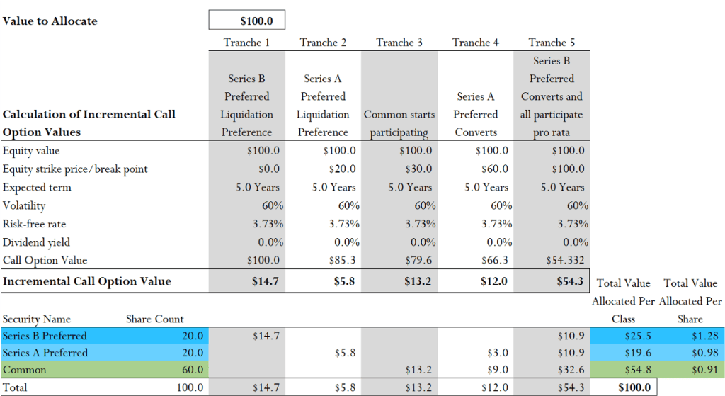
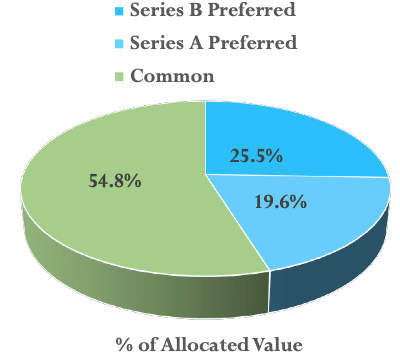
The Option Pricing Method, also outlined by the AICPA, is widely used in valuations of multi-class equity that are not expected to sell immediately. It is forward-looking and examines the optionality inherent in each tranche of participation, capturing the incremental call option value at each breakpoint.
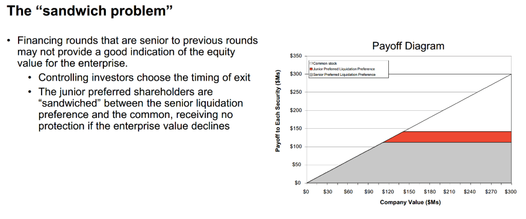
The OPM has important limitations. It is best suited to structures with only one class of liquidation preference. The AICPA PE/VC Guide notes that the OPM is not ideal for estimating the relative value of senior and junior preferred classes and does not consider the future funding requirements of companies anticipating future losses. Because the OPM includes a time to liquidation, it also carries an implied return, and it typically implies low relative risk and return in the first tranches, which may not reflect reality.
Method 3 of 3: Scenario Based Methods
Scenario-based methods are forward-looking approaches that model one or more possible future outcomes. The AICPA guidance directs that a fund should determine how each class of equity would participate in future distributions from a sale or liquidity event, and estimate the fair value of each class based on its future payoffs at the time of that event. The guidance deliberately does not prescribe specific techniques, leaving room for well-supported methods.
The Discounted Future Proceeds Method
The Discounted Future Proceeds Method is a Scenario Based Method developed by Deal Valuation. It is best used in valuations that assume an exit and the need for future financing. The critical factors it considers include the time to a sale or liquidation event, the estimated sale or IPO value, the future capital needed to achieve that value, and the required return for each equity class participating.


The DFPM draws a direct connection between the business enterprise valuation and the equity allocation. It combines the discount rate and sale value from a Discounted Cash Flow analysis with the natural equity allocation logic of the Current Value Method. By determining a discount rate for each tranche of participation, the value of each equity class can be directly correlated with the path and risk of management’s projections.
How the DFPM Works
STEP 1
Allocate the Future Sale Value
Using the future sale value from a DCF and the liquidation preferences due at that future date, the DFPM performs a Current Value Method allocation as of the exit, distributing the future proceeds across each tranche according to its participation.
STEP 2
Discount Each Tranche to Present Value
The future proceeds are then discounted back to present value. Because each tranche has a different priority and therefore a different risk profile, each is discounted at a rate specific to its required return. The discount rate for Tranche 1 is selected first, with incremental premiums added for each more subordinate tranche.
STEP 3
Reconcile to the DCF
The present value allocated to the final participating tranche is adjusted so that the sum of all present values equals the present value indicated by the DCF. This reconciliation considers both the required return implied by the final tranche and the total weighted-average return across all classes relative to the DCF discount rate.
The weighted average return, or WAR, is calculated by multiplying the percentage of value allocated to each class by the implied return for that class. A correctly constructed DFPM produces a total WAR comparable to the discount rate used in the DCF, confirming that the allocation is internally consistent.
The Four Key Drivers of the DFPM
Time to Exit
Should match the exit in the DCF and extend to a realistic exit profile.
Returns per Tranche
The initial rate and the incremental premiums for each subordinate tranche.
Exit Value
Same as the DCF, with consideration of interim profits and losses.
Final Tranche and Conclusion
Tied back to the DCF or back-solved to the latest financing round.
PRACTICAL INSIGHTS

Higher exit values drive higher required returns for senior tranches. The required return for the first tranche should consider any senior instruments, such as outstanding debt or earnouts. The required return for the final tranche reflects the risk of the value allocated at the future sale date, not all potential value, and can vary widely when only small amounts are due in that tranche. Incremental premiums should reflect the reality of multiple layers of risk across the capital stack, all driven by one underlying business. Running multiple DFPMs to model different paths to exit creates a robust Scenario-Based Method.
The Fourth Method: Hybrid
The AICPA guidance also describes a fourth approach, the Hybrid Method, which combines more than one method, specifically the OPM and a Scenario-Based Method. Using the DFPM as the Scenario-Based component, a Hybrid analysis weights multiple scenarios to arrive at a final allocation.
Guidance from the AICPA, the ASA, and the SEC all indicates that valuations must consider future events, multiple scenarios, and the risk and return associated with each. The DFPM provides a solid foundation for valuations involving start-up and expansion-phase companies with multi-class capital structures.

Choosing the Right Method
Current Value Method
Best for: imminent sale or liquidation
Key limitation: ignores time to exit and unequal required returns
Option Pricing Method
Best for: single class of liquidation preference, future exit
Key limitation: struggles with multiple preferred classes and future funding needs
Scenario-Based Method / DFPM
Best for: multi-class structures with an exit and future financing needs
Key limitation: requires well-supported discount rates per tranche
Hybrid
Best for: blending probability-weighted scenarios
Key limitation: more complex to build and support